

Standard column filters in Google Sheets work well for some datasets, but they’re hidden inside menus, require edit access to use, and filter a single table at a time. Slicers sit on top of your sheet as floating, clickable controls that anyone can use (regardless of access). They also update every connected pivot table and chart on the sheet the moment you make a selection. Here’s how to add slicer to Google Sheets, customize how it looks, and use some advanced options for using it.
How to Add Slicer to Google Sheets
Slicers work best when your data is in a structured table where you have column headers in the first row, no merged cells, and no blank rows breaking up the data. If your spreadsheet already has a pivot table or chart built from a defined range, the slicer will pick up that range automatically. If you’re working with a flat data table, you can click anywhere inside the table before adding the slicer so Google Sheets can identify the correct range on its own.
Step 1. Click on any cell within the data range you want to filter. If you want to attach the slicer to a chart or pivot table you’ve already built, click on the chart or pivot table instead. Make sure to organize your data with column headers in the first row, with no blank rows or merged cells.
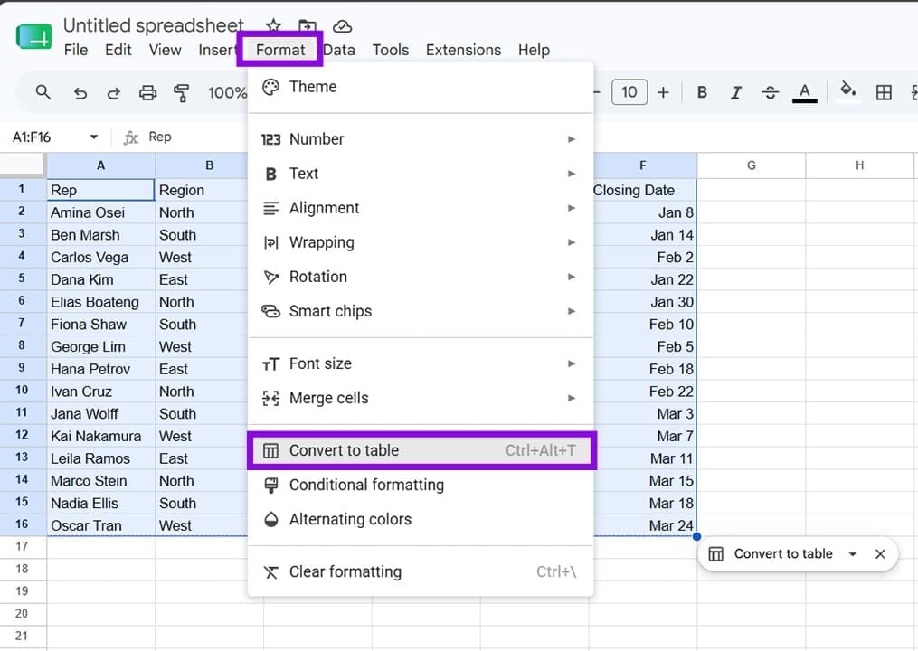
Step 2. Go to the top menu, click “Data,” and choose “Add a slicer.”
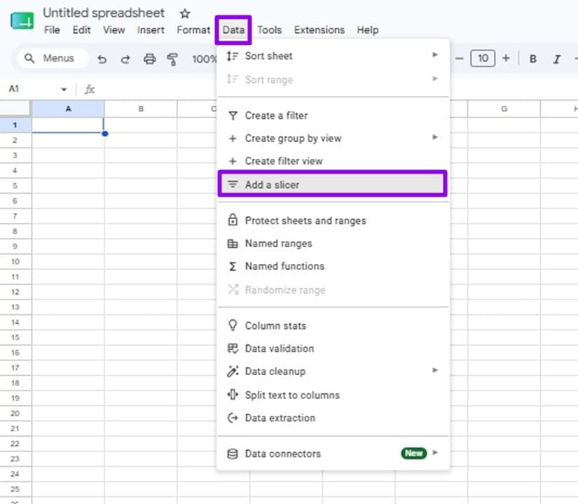
Step 3. In the sidebar, under the Data tab, you’ll see a data range field. Google Sheets usually fills this in based on your selection. If it’s blank or wrong, click the grid icon next to the field and select the correct range, or type it in manually (for example, A1:F216).
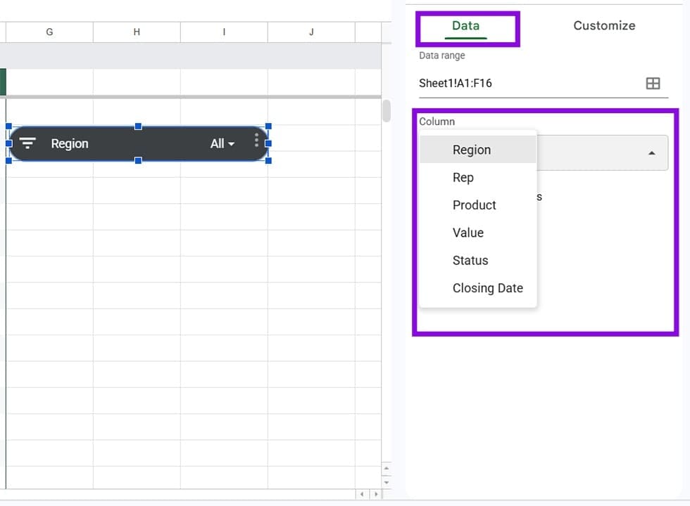
Step 4. Still in the Data tab, open the Column dropdown and choose which column the slicer should control.
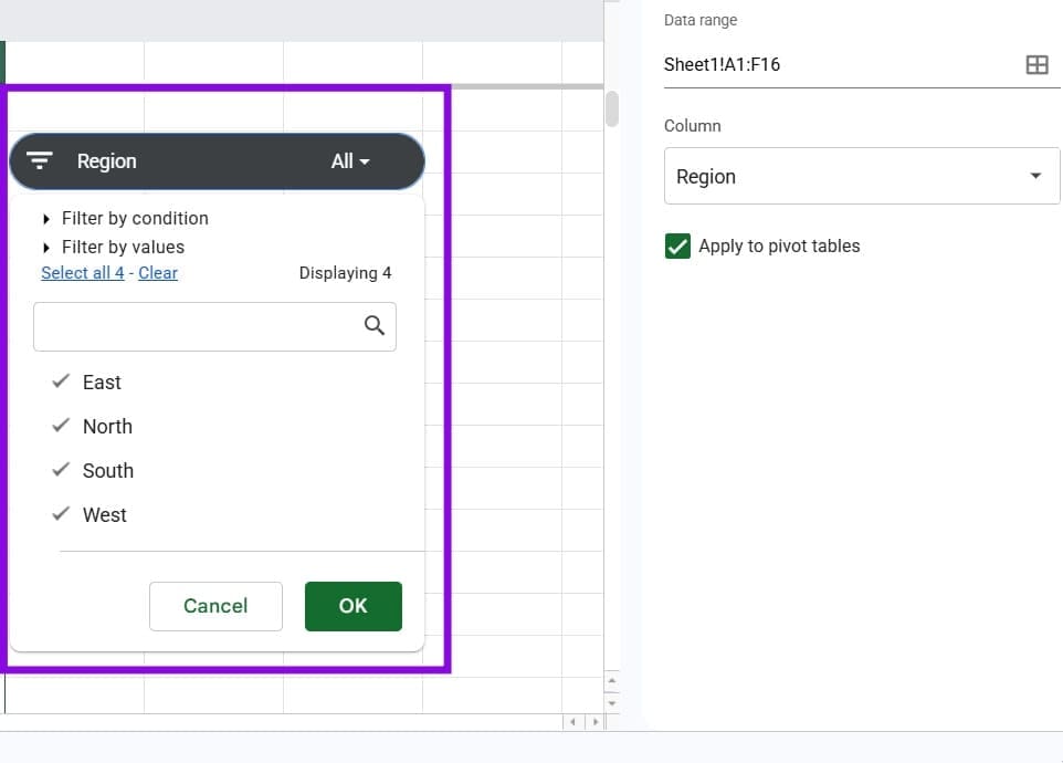
As for how to use slicer in Google Sheets, you need to click on its dropdown arrow. You’ll see a list of all unique values in the column you chose, and you can check or uncheck data.
How to Customize the Slicer’s Appearance
Once a slicer is on your sheet, you can adjust how it looks.
To open the customization options, double-click on the slicer and go to the “Customize” tab on the sidebar. From there, you can change the slicer’s title – it defaults to the column name, but you can rename it to something more readable – the title font, size, and formatting, the background color of the slicer box, and the text color.
To resize the slicer, click on it to select it and drag the handles on its edges.
Once you’ve styled a slicer the way you want it, you can use it as a template for additional slicers by clicking the three-dot menu and selecting “Copy slicer,” then pasting it onto the sheet. The copy inherits the same appearance settings, so you only need to change the column it filters.
How to Add Multiple Slicers for Multi-Column Filtering
One slicer controls one column. For example, if you want to filter your data by Region and by Product at the same time, you need two separate slicers.
To add a second slicer for a different column, repeat the same process as with the first and choose a second column for it, or create a copy of the existing slicer.
There’s no hard limit on how many slicers you can add, but most tables will cap out at three or four. Beyond that, consider whether a filter view or a pivot table with report filters would serve the use case better.
Was this helpful?
Last updated on 28 May, 2026
Read Next
 3 Ways to Add Dates Automatically in Google Sheets
Method 1: Automatically Enter the Current Date Let's start by automatically entering today's date using the Google Sheets date function called TODAY().
3 Ways to Add Dates Automatically in Google Sheets
Method 1: Automatically Enter the Current Date Let's start by automatically entering today's date using the Google Sheets date function called TODAY().
 3 Ways to Add or Remove Gridlines in Google Sheets
Method 1: Add or Remove Google Sheets Gridlines From View Menu The easiest way to remove or add gridlines from Google Sheets is using the View menu.
3 Ways to Add or Remove Gridlines in Google Sheets
Method 1: Add or Remove Google Sheets Gridlines From View Menu The easiest way to remove or add gridlines from Google Sheets is using the View menu.
 How to Add and Customize a Trendline on a Chart in Google Sheets
How to Add a Trendlline in Google Sheets The purpose of a trendline is to highlight the patterns in data.
How to Add and Customize a Trendline on a Chart in Google Sheets
How to Add a Trendlline in Google Sheets The purpose of a trendline is to highlight the patterns in data.
 4 Ways to Create Desktop Shortcuts for Google Docs or Sheets
Note: Ensure that the Google Docs or Sheets website is open in the browser if you want to add shortcuts to any particular file.
4 Ways to Create Desktop Shortcuts for Google Docs or Sheets
Note: Ensure that the Google Docs or Sheets website is open in the browser if you want to add shortcuts to any particular file.
 Top 9 Google Sheets Budget Templates for Finance Tracking
Managing money can be tricky sometimes.
Top 9 Google Sheets Budget Templates for Finance Tracking
Managing money can be tricky sometimes.
 2 Best Ways to Import Questions Into Google Forms From Google Sheets
Typically, when you create a Google Form, you need to perform several steps.
2 Best Ways to Import Questions Into Google Forms From Google Sheets
Typically, when you create a Google Form, you need to perform several steps.
 How to Insert a Date Picker in Google Sheets and Google Docs
Google Sheets and Google Docs provide a free, online alternative to Microsoft Office, along with unique features.
How to Insert a Date Picker in Google Sheets and Google Docs
Google Sheets and Google Docs provide a free, online alternative to Microsoft Office, along with unique features.
 4 Ways to Fix Formulas Not Working in Google Sheets
Fix 1: Modify Spreadsheet Calculation Settings Incorrect calculation settings are another reason Google Sheets formulas may not work or update.
4 Ways to Fix Formulas Not Working in Google Sheets
Fix 1: Modify Spreadsheet Calculation Settings Incorrect calculation settings are another reason Google Sheets formulas may not work or update.
The article above may contain affiliate links which help support Guiding Tech. The content remains unbiased and authentic and will never affect our editorial integrity.