

Excel is a versatile spreadsheet program, with many functions that help in the workplace and for home organization. You can use Excel to add up and subtract many values, including the number of days someone has been working, going to the gym, or just about any other activity.
When you want to be precise about working days, though, you need to use the Excel NETWORKDAYS function to calculate working days in Excel, excluding weekends and holidays. Read the full guide below to learn how.
Reasons to Calculate Working Days in Excel
If you’re calculating pay, benefits, or time off for team members, it helps to only include working days so you don’t have to manually adjust for weekends or holidays.
Similarly, if you like to keep a spreadsheet showing hours you’ve worked, the ability to automatically remove your non-working days from your total is a real time-saver.
Excel NETWORKDAYS Function Explained
To calculate the number of days between two dates, you can use a simple subtraction formula or either the DATEDIF or DAYS function. However, these methods won’t automatically exclude weekends or holidays.
Helpfully, Microsoft Excel has a function called NETWORKDAYS, which is designed for the exact purpose of excluding non-working days. As the name suggests, it helps you calculate net working days, excluding weekends and, in some cases, vacation days.
Calculate Working Days in Excel: Step-by-Step Guide
Step 1. Open your workbook that has date-related data. Make sure you add a start date and an end date for each entry, plus a column for the total workdays.
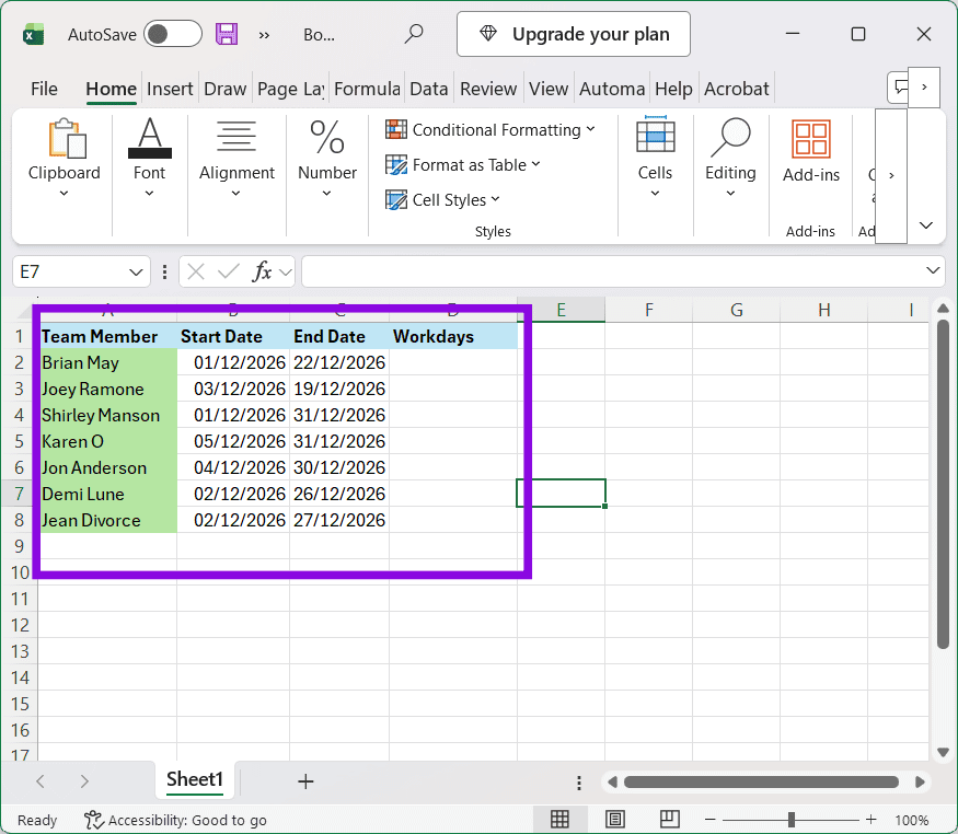
Step 2. Create your formula in the first Workdays cell. Click the Insert Function (fx) button next to the formula bar to open the function selection dialog.
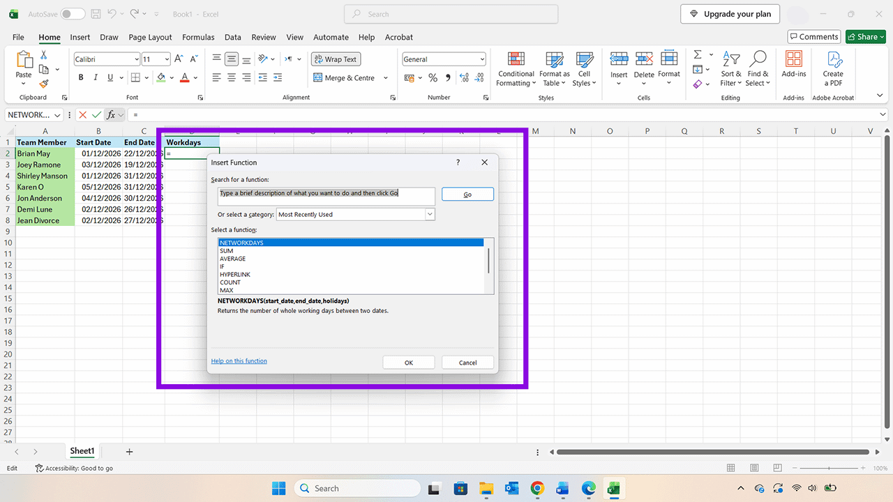
Step 3. Select “NETWORKDAYS.” If you don’t see it in the list of common functions, use the search box to find it. Press “OK” to open the Function Arguments dialog.

Step 4. Enter the cell number of the first working day into the Start date box. Put the cell containing the last day for the same person into the End date box. Note: You can click on the relevant cells as well as type the digits manually.
You will see the function appear in the text bar like this:
=NETWORKDAYS(B2,C2)
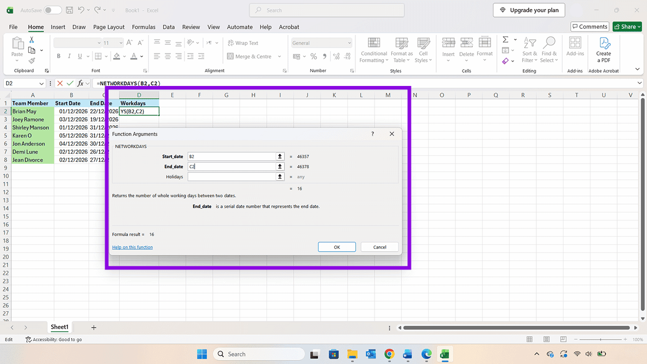
Step 5. Press “OK” to see the number of working days appear in the relevant cell.
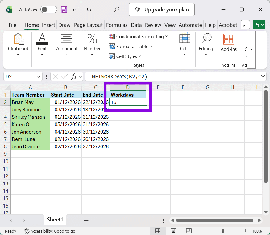
Step 6. You can now hover over the bottom-right corner of that cell and, when the black plus sign appears, drag it down to replicate that function across all the cells of the Workdays column.

Step 7. You can now see workdays minus any weekends. But as you may have noticed, these shifts are in December, where there are several holidays, depending on where you live or work. There may also be dates when your company is closed for other reasons. To include holidays, create a new dataset of those dates in a separate column.

Step 8. Use the NETWORKDAYS function as before, but this time, amend it to include the holiday dates like this:
NETWORKDAYS(B2,C2, $A$11:$A$15)
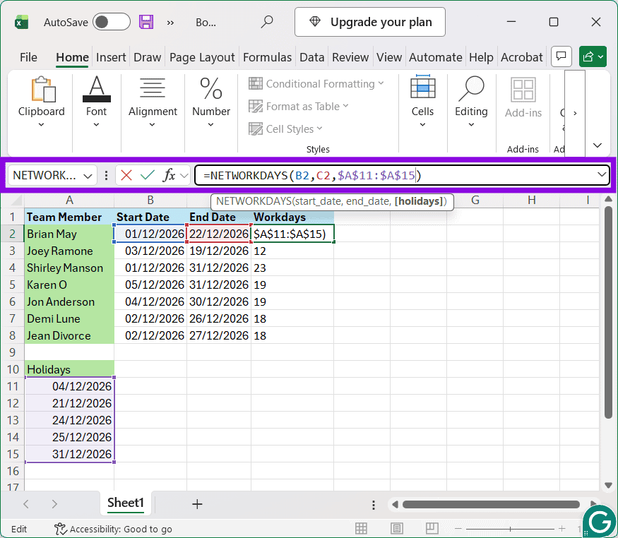
Step 9. Press “Enter,” drag the formula to the other cells, and you will see the amended Workdays column showing only working days, minus both weekends and holidays.

Was this helpful?
Last updated on 09 November, 2026
Read Next
 How to Stop Excel Changing Fractions to Dates
Despite its many advantages and benefits, Excel doesn’t always behave as users would want or expect.
 3 Ways to Add Dates Automatically in Google Sheets
Method 1: Automatically Enter the Current Date Let's start by automatically entering today's date using the Google Sheets date function called TODAY().
 How to Video Chat Between Android and iPhone
How to Use FaceTime on Android Devices Android users can be a part of FaceTime conversations by accepting an invitation from iOS users.
 How to Remove Extra Space Between Words in Microsoft Word
Method 1: Find and Delete Extra Spaces in Microsoft Word Using Find and Replace The first obvious way is to do it manually since you wouldn't want automation to cause
 How to Use Microsoft Edge Drop Feature to Share Files Between Devices
How to Send Files From Your Desktop Using Microsoft Edge Drop Microsoft Edge’s Drop feature is only available in version 110.0.1587.41 or later.
 How to Switch Between KM and Miles in Google Maps and Apple Maps
How to Change Kilometers to Miles in Apple Maps To change KM to Miles (or vice versa) on iPhone, iPad, and Mac, all you need to do is change your
 4 Fixes for Spotify Not Syncing Between Mobile and Desktop
Basic Fixes Use the same account on multiple devices: Sometimes you don't realize, but you must have the same account on all your devices.
 What’s the Difference Between Album and Folder in Photos
You may have seen the terms albums and folders in Google Photos and Apple Photos.
The article above may contain affiliate links which help support Guiding Tech. The content remains unbiased and authentic and will never affect our editorial integrity.