3 Ways to Format Tables in Google Sheets

Quick Tips

• Liven up your data with custom headers, rows, or alternating band colors.
• Apply pre-designed themes for a cohesive and professional look with a single click.
• Unlock more formatting options with the Table Styles Add-on, offering a wider variety of borders, fonts, and effects.

Method 1. Change Table Colors

Step 1: Open a spreadsheet in Google Sheets.

Step 2: Once you are done adding entries and making tables, click on Format at the top.

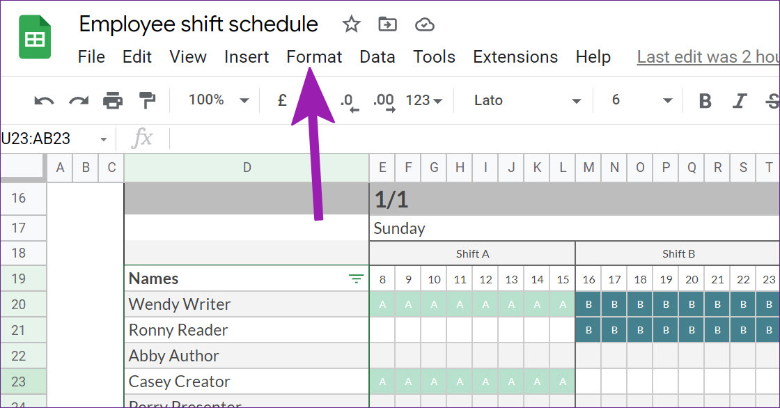
Step 3: Select Alternating colors, and it will open a side menu.

Step 4: Click on the little icon beside the current range and select a custom range to apply colors.

Step 5: Select one of the default styles, and you will instantly see a new style in action.

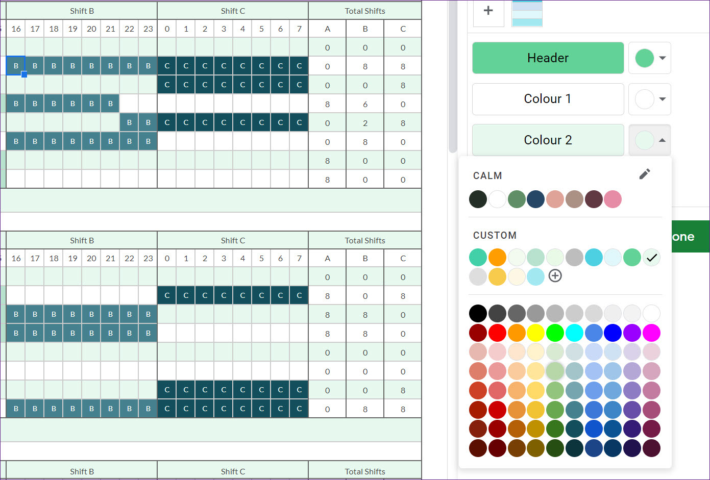
You can even change the header, color 1, color 2, and footer theme to your preference. Once you make changes in default styles, it will be saved as a custom theme so that you can use it in the future with a single click. Hit the Done button and enjoy your spreadsheet in a colorful avatar.

Method 2. Use Themes

Step 1: From Google Sheets, select Format in the menu bar.

Step 2: Click on Themes from the drop-down menu.

Step 3: Check a bunch of default themes from the right sidebar.

Step 4: Select your preferred theme and check the new color in action.

If you don’t prefer anything from the list, select any theme and click on Customize at the top.

The following menu will help you change font type, text color, chart background, color, hyperlink color, and edit different accent colors in a theme. Hit the Done button, and you are good to go.

Method 3. Use Table Styles Add-on

Using a third-party add-on called Table Styles, you can change the look of the spreadsheet on the go. First, we will show you how to install Table Styles in your Google Sheets account and check the add-on in action.

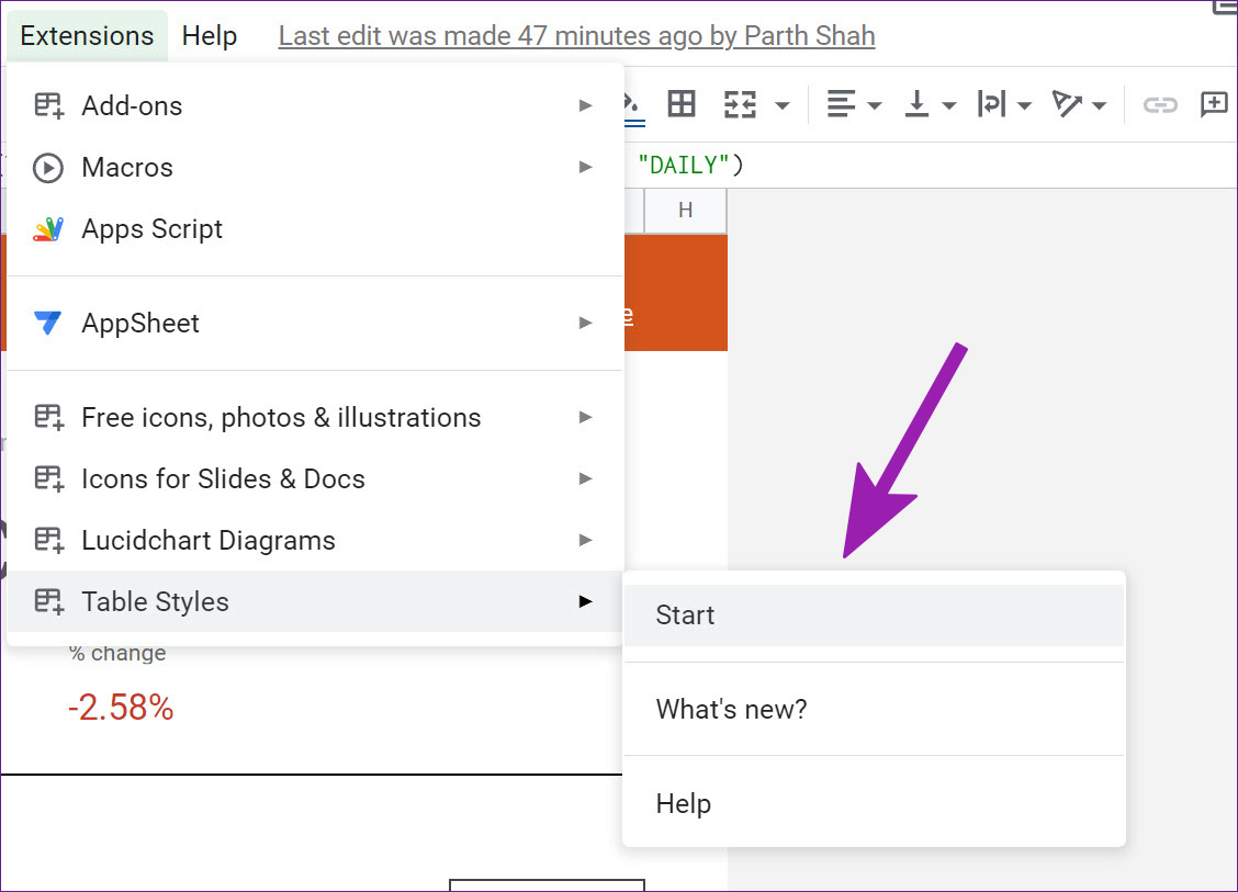
Step 1: From Google Sheets, click on Extensions at the top.

Step 2: Open the Add-ons menu and select Get add-ons. It will open the Google Workspace Marketplace.

Step 3: Use the search bar at the top and search for Table Styles.

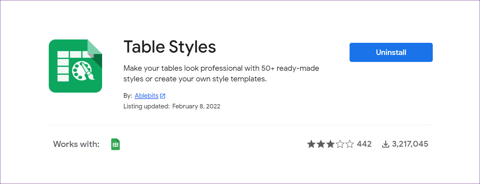
Step 4: Install Table Styles in Google Sheets.

Now that you have installed Table Styles, let us show you how to use the add-on to format tables in Google Sheets.

Step 5: Once you open a spreadsheet, select Extensions in the menu bar.

Step 6: Expand Table Styles > click on Start.

You will see Table Styles in action from the right-side menu. Unlike the default Alternating colors option in Google Sheets, Table Styles won’t automatically detect a table in Sheets. You need to select the cell range manually. We have selected B27:F38 to format in Google Sheets in the example below.

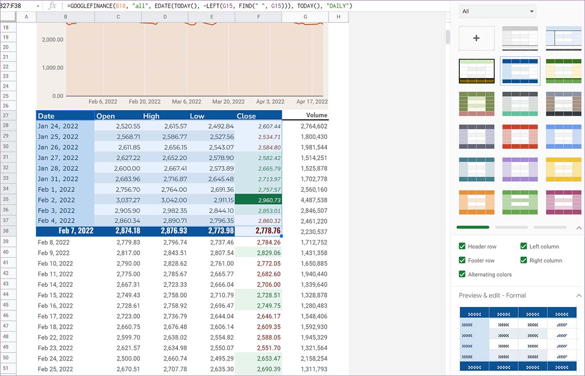
Select one of the themes from Table Styles. The extension offers several styles to choose from. You can change the style with lighter, darker, or contrast colors.

Besides changing the header row and footer and implementing alternating colors, Table Styles will change the left and right column colors.

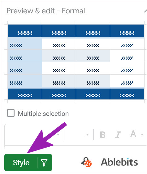
You can expand the Preview & edit option and check the format in action before applying it to Google Sheets. Once you are satisfied with the preview, hit the Style button at the bottom.