How to Make Excel Tables With Multiple Header Rows Easier to Use

Quick Tips

• Multiple header rows can be a disaster for understanding and formatting data.
• It’s easy to fix thanks to Power Query.
• First, format your dataset into a table, then open the Power Query editor to fix the problem.

Sometimes we complicate our lives, and that includes Excel spreadsheets. Sometimes they’re a little too detailed for our own good. Having multiple headers in a spreadsheet can do more harm than good when it comes to proper organization.

But before you dump everything in the Recycle Bin, the good news is that fixing this problem is pretty simple to do. In this article, we’ll be showing you how to do it.

Fix Multiple Header Rows in Excel With Power Query

It may seem like a good idea to add more specificity by including two or more header rows to your columns. But the truth is that not only can it quickly become confusing to read and understand, but formatting your data and calculating formulas can become problematic, especially if you have multiple columns with the same name.

The quickest and most convenient way to fix this problem, apart from manually deleting the headers yourself (and even that might prove problematic in some cases), is to use Power Query to sort things out.

Setting Up Your Table

Before you can use Power Query to organize things, you’ll first need to set up your data set as a table. Here’s how:

Step 1. Open up your spreadsheet and click anywhere in your dataset.

Step 2. Navigate to the “Home” tab and click the “Format as Table” button on the ribbon.

Step 3. Select the layout for your table from the list and click to select it.

Step 4. A small window will pop up. If it isn’t done already, check the box next to “My table has headers.” Ensure the automatic range selection encompasses all the data your set. Adjust in the dialog box if not. Click “OK” to confirm.

Step 5. Because your table has two header rows, you’ll need to initially remove the automatic header formatting. In the “Table Design” tab, uncheck the box next to “Header Row” in the “Table Style Options.”

Using Power Query

Now that your table is set up, it’s time to finish the job with Power Query:

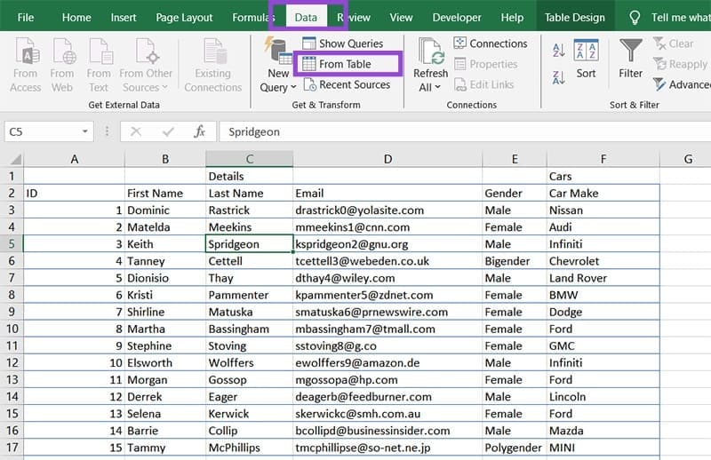
Step 1. Head to the “Data” tab and click anywhere in your table.

Step 2. Click the “From Table” or “From Table/Range” (depending on your version) on the ribbon.

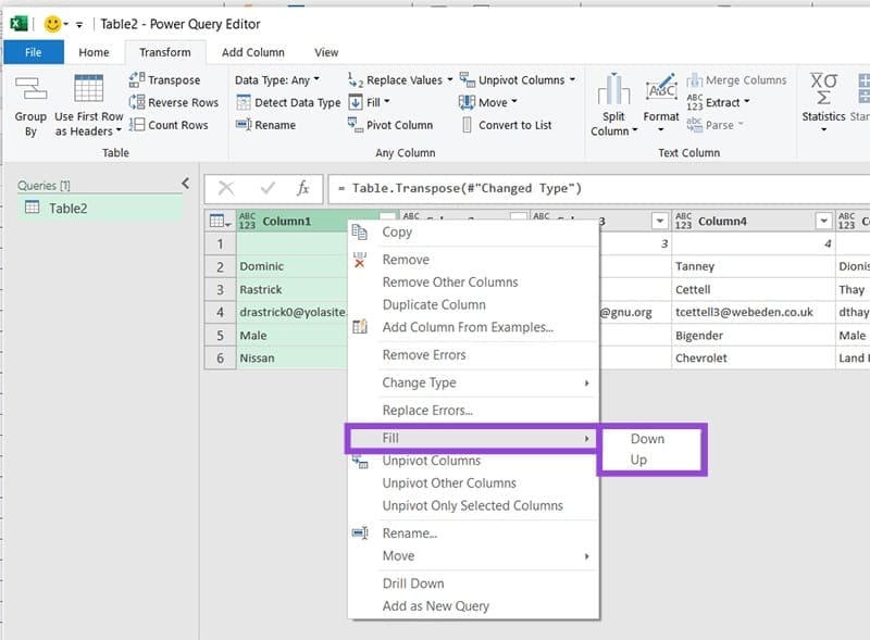
 Step 3. The Power Query Editor will open. Head to the “Transform” tab and click the “Transpose” option to flip the rows into columns and vice versa.

Step 4. Fill in any blanks in your extra header rows (now columns). These will be filled with the “null” value.

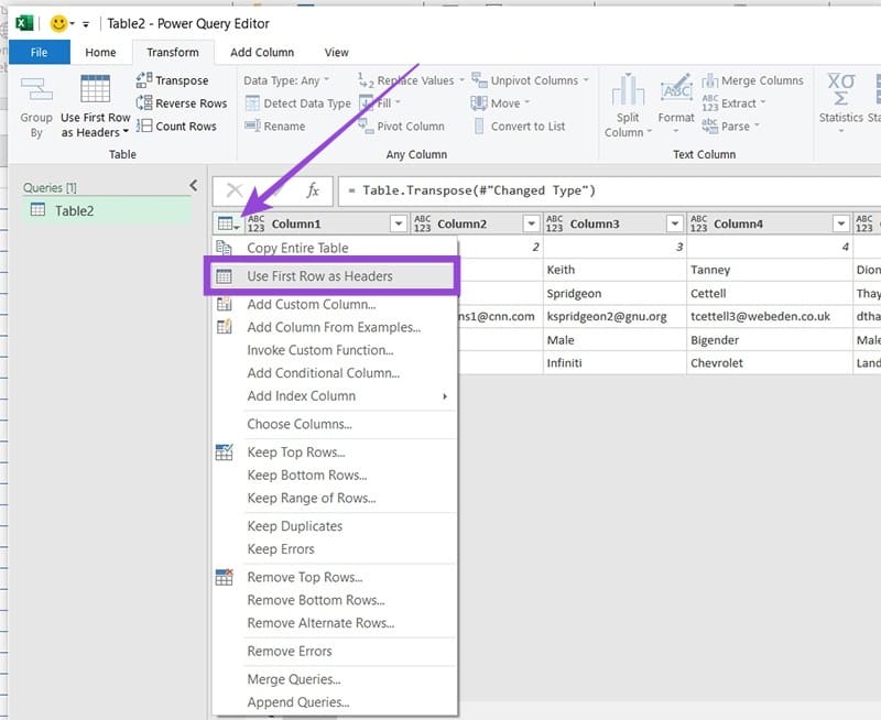
Step 5. Now flatten the top row into a header by clicking the Table icon in the top left and selecting “Use the First Row as Headers.”

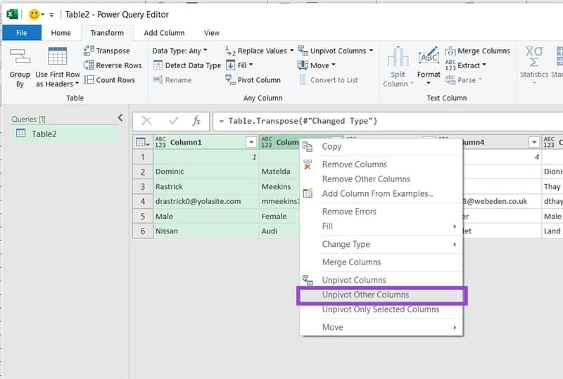
Step 6. To add these rows to the other headers, select them (Shift + Click the columns you want to unpivot) and then right-click those same headers. Select “Unpivot Other Columns.”

Step 7. The Row Headers will now be listed as a data type of their own.

Step 8. Rename the columns, then click “Close & Load” in the “Home” tab to finish the process.