When working with a large spreadsheet in Excel, it can be challenging to spot duplicate entries. Besides, you might also accidentally enter the same piece of information twice. To quickly identify these errors and ensure that your data is clean and accurate, it is better to highlight duplicates in Excel with a few clicks. This can save you plenty of time and frustration in the long run.

There are multiple ways to highlight duplicates in Excel, and the method that you use will depend on the data that you are working with. In this article, we are going to show you all the different ways to get the work done efficiently. Let’s start.
Things to Keep In Mind When Handling Duplicate Values
- You must determine whether the duplicates are exact or approximate. Exact duplicates are exact copies of a record, while approximate duplicates may have some slight variations.
- It is essential to determine whether the duplicates are within the same or different datasets. If they are within the same dataset, you can simply delete the duplicates. However, if the duplicates are across different datasets, you may have to keep both copies and merge them.
- Finally, it is important to consider the impact of the duplicates on any analyses that will be performed. Duplicates can introduce bias and skew results, so it is important to be aware of this when dealing with them.
How to Find Duplicates in Excel
Below are some of the ways to find duplicates in Excel:
- Use COUNTIF – This built-in function counts the number of cells that satisfy the criteria you specify. It counts the number of times each value appears in a column. A value is considered a duplicate if it appears more than once.
- Use the Conditional Formatting feature – This feature allows you to highlight cells that meet certain criteria. So, to find duplicates, you can use conditional formatting to highlight cells that contain duplicate values.
- Use a VBA macro – This method is a bit more advanced and powerful. There are many different ways to write a macro to find duplicates, so I won’t go into detail here. But, if you are interested in learning how to write a macro, there are many resources available online.
No matter which method you use, finding duplicates in Excel can be helpful to clean up your data. Let’s explore the most effortless methods step-by-step.
Highlight Duplicates From Individual Rows/Columns in Excel
To highlight duplicates and non-unique values, follow these steps.
Step 1: Open Spreadsheet with Microsoft Excel.

Step 2: Now, select the dataset in which you want to check for duplicates. Don’t forget to include the column header in your selection.

Step 3: Under the style section, select conditional formatting.

Step 4: Select Highlight Cell Rules and go to Duplicate Values.
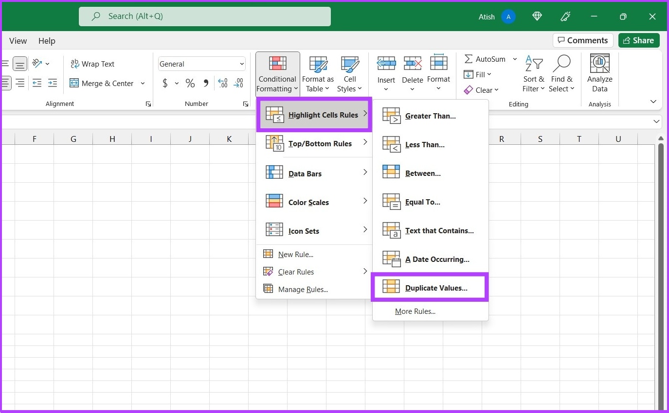
Step 5: Click on the first drop-down menu and choose Duplicate. In the next drop-down, pick the formatting you want to use to highlight the duplicate entries. Now, click on OK.
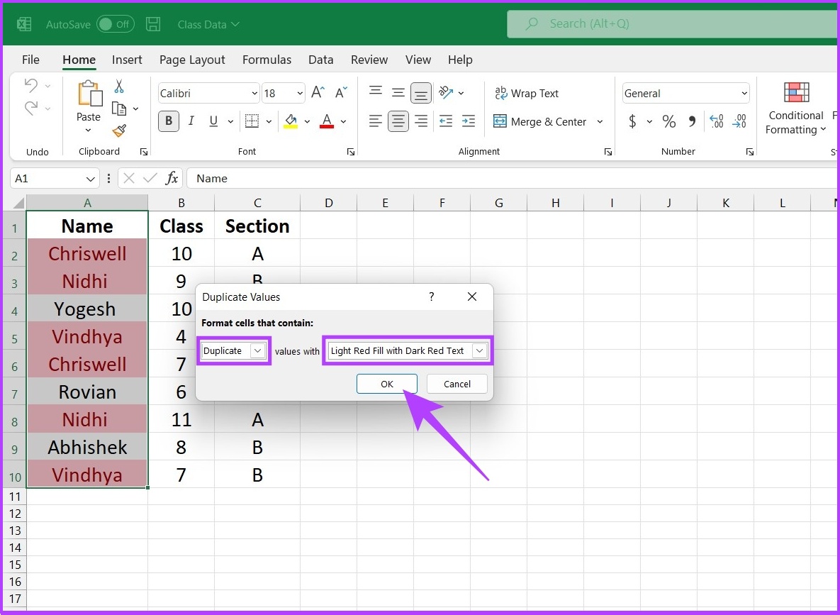
There you go. On your spreadsheet, you will find that Excel has highlighted the duplicate entries. Wasn’t it simple? That said, if you are struggling with the formatting of tables, check out these best ways to format table data in Microsoft Excel.
How to Use Excel Formula to Find Duplicate Columns or Rows
COUNTIF is one of the most commonly used Excel formulas for highlighting duplicates. As discussed above, it is primarily used to count the number of cells that appear within a defined range and meet the predefined criteria. Besides, it also outstands the contemporary ‘Conditional Formatting’ function as it allows the user to define the command, unlike conditional formatting, which only picks out duplicates.
Using the COUNTIF function, one can not only highlight duplicates but also triplicates and other repetitive values. Moreover, it also eases up highlighting a whole row based on duplicate values in one specific column, multiple columns, or all columns.
Syntax: =COUNTIF (range, criteria)
The range defines the range of cells where the formula needs to be applied and the criteria define the basis that needs to be applied to identify duplicates.
How to Highlight All Values in Spreadsheet
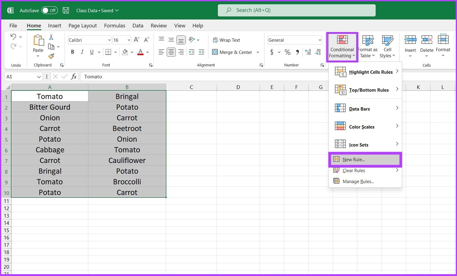
Step 1: Select the range of cells. Now, go to the Conditional Formatting function in the Home tab and select New Rule.
Step 2: Choose the option ‘Use a formula to determine which cells to format’.
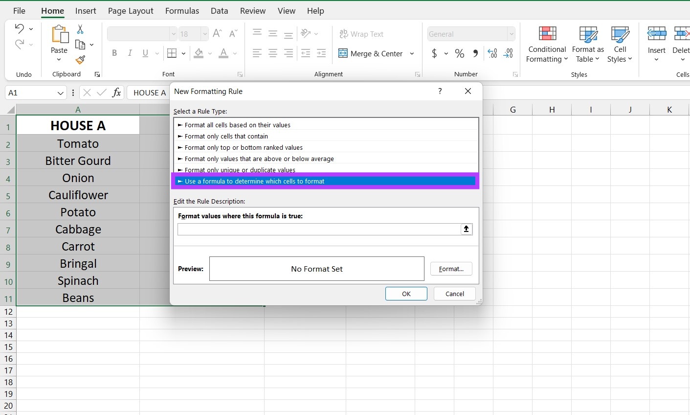
Step 3: Now, feed the formula using range and criteria and click on OK.
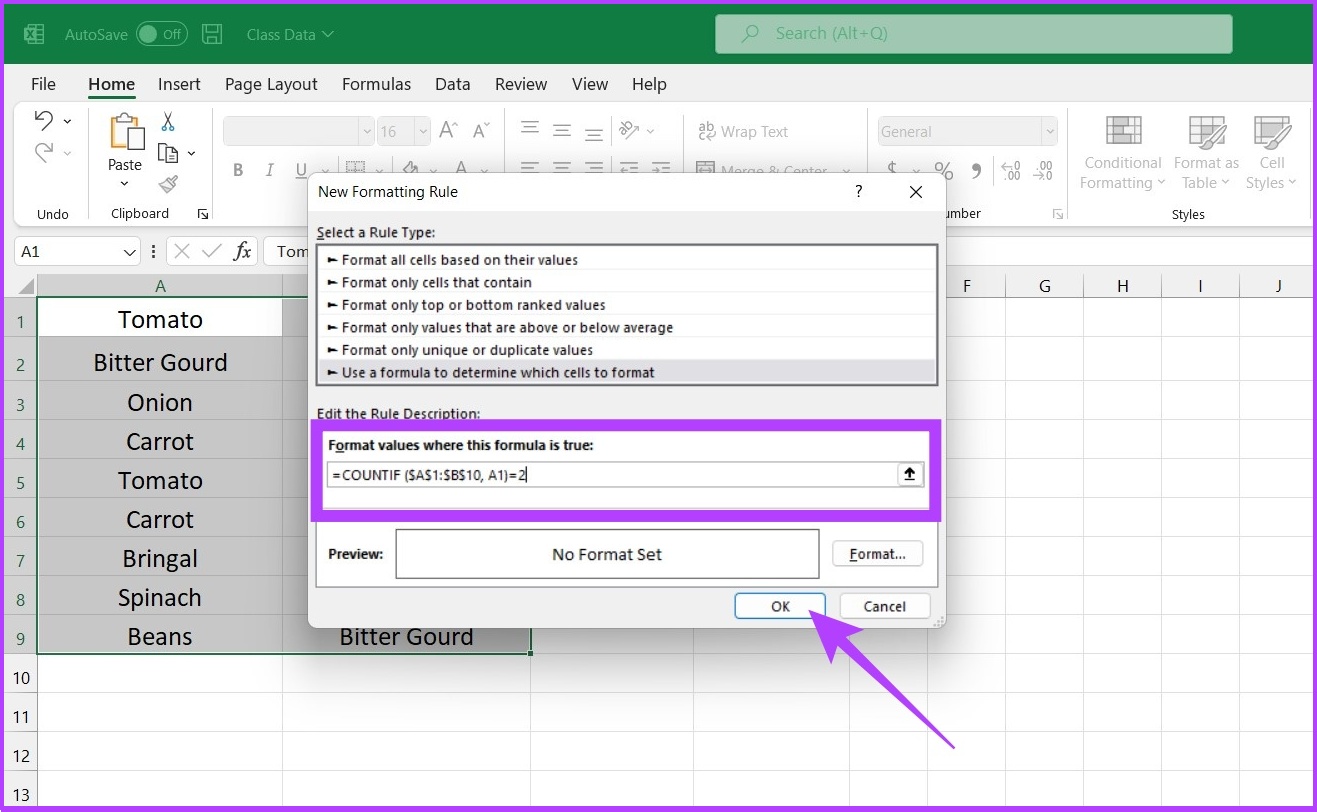
For example: ‘=COUNTIF ($A$1:$B$10, A1)=2’
In this example, ($A$1:$B$10) defines the range A1:B10 for Excel, whereas A1 is the criterion, meaning Excel will compare and identify the same value as that in cell A1 to the highlighted cells, i.e., A1:B10. The number after equal to determines the number of times the value in A1 should be repeated in A1 to B10 to be highlighted.
Step 4: Once you have determined the formula, select the defined range and click on the bottom icon to set up the formatting style.
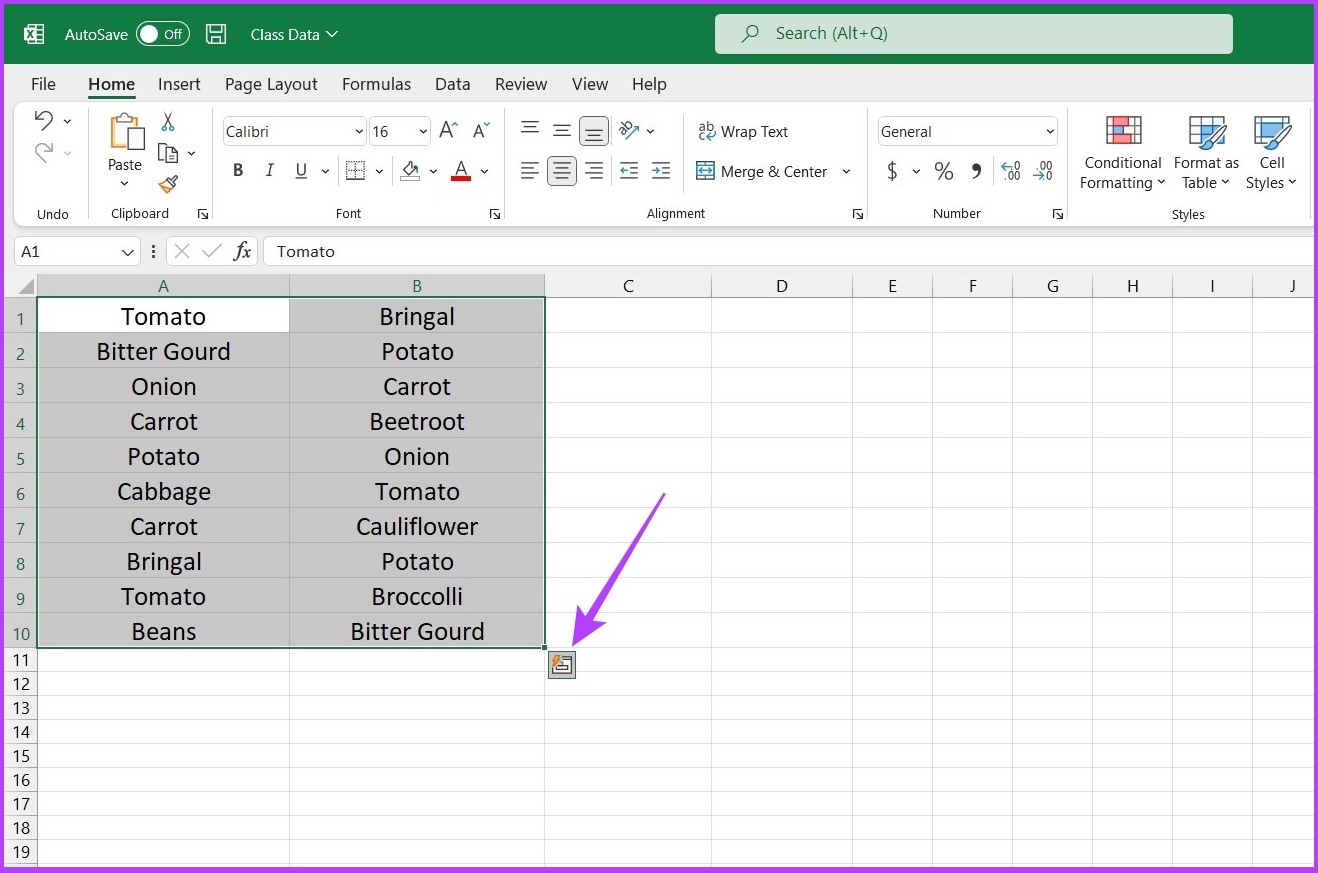

That’s it. If any value appears twice, Excel will highlight the cell.
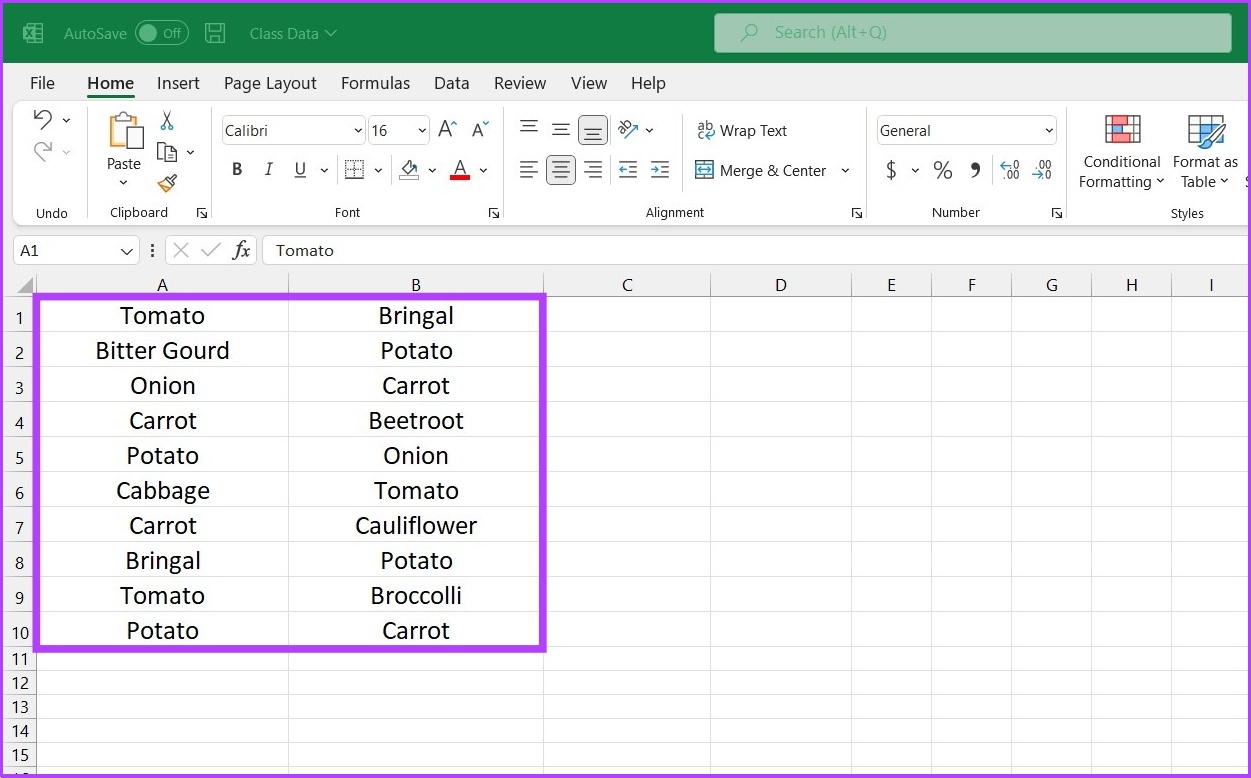
If you notice, Bringal & Carrot were not highlighted, as they don’t appear more than twice. You can amend the COUNTIF formula to get the results you want.
For instance, you can change the formula to =COUNTIF ($A$1:$B$10, A1)= 3 to highlight all triplicate values. Or change the formula to = COUNTIF ($A$1:$B$10, A1) > 3 to highlight cells that appear more than thrice.
Highlight Duplicates in Rows on Excel
The built-in highlighter duplicates values only at the cell level. That said, if you want to highlight an entire row of duplicate values, you need to tweak the COUNTIF function to achieve your desired result.
Step 1: Firstly, select the cells to check for duplicates.
Step 2: Go to the Conditional Formatting function under the Style section and Select New Rule.
Step 3: Choose the option ‘Use a formula to determine which cells to format’.
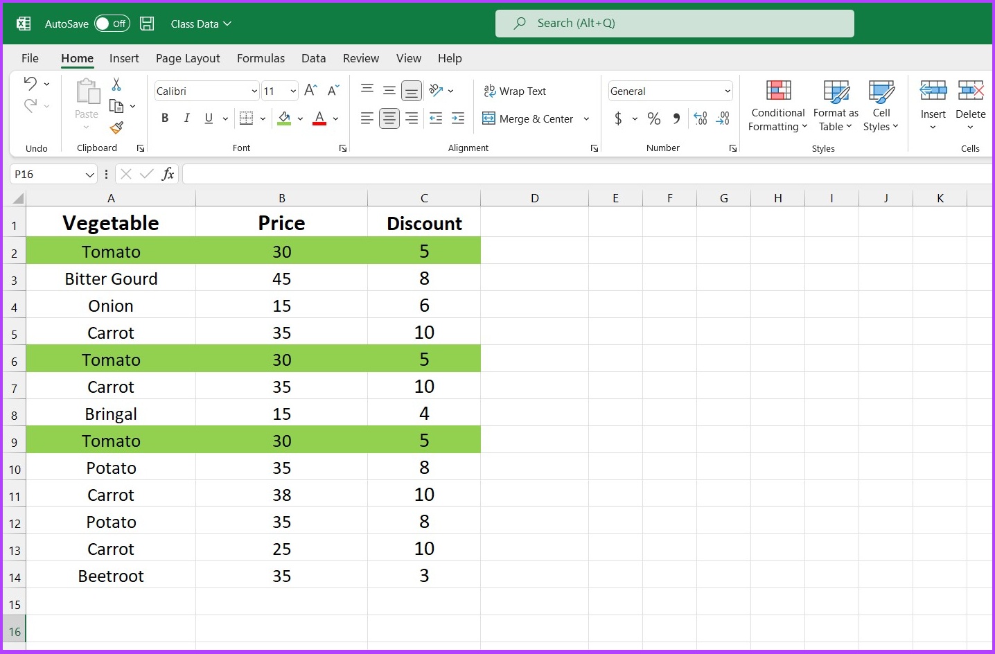
Step 4: Enter the formula i.e. ‘= COUNTIFS ($A$2:$A$14,$A2,$B$2:$B$14,$B2,$C$2:$C$14,$C2) = 2’

There you go. Excel will produce the result based on your query.
Mind you, the COUNTIFS function works like the COUNTIF function. If you want to identify triplicates, substitute ‘2’ from the above formula with ‘3’. You can also set criteria as ‘>1’ or ‘<3’.
Example: ‘= COUNTIFS ($A$2:$A$14,$A2,$B$2:$B$14,$B2,$C$2:$C$14,$C2) = 3’
If you are facing an issue while using Excel on Mac, check these best ways to fix Microsoft Excel not opening on Mac.
How to Remove Duplicate Values in Excel
Not only can you highlight the duplicate dataset, but you can also easily remove it using Excel. Here’s how to do it.
Step 1: Firstly, select the dataset you want to remove duplicates from. Don’t forget to select the column header along with the selected column.
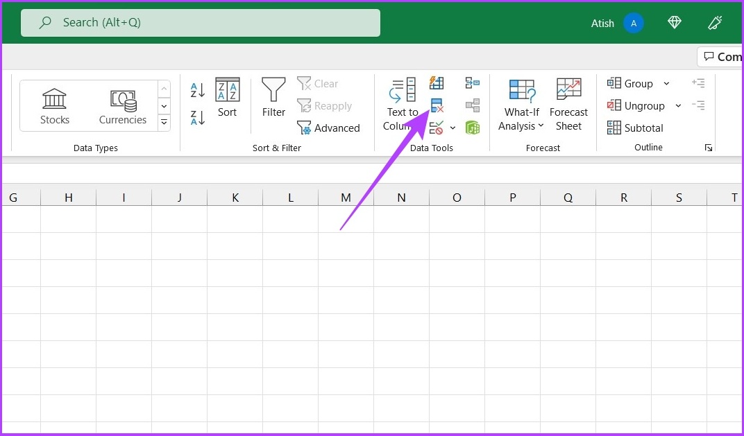
Step 2: In the Excel menu at the top, click the Data tab.

Step 3: Now, from the Data Tools section, click on the Remove Duplicates icon.
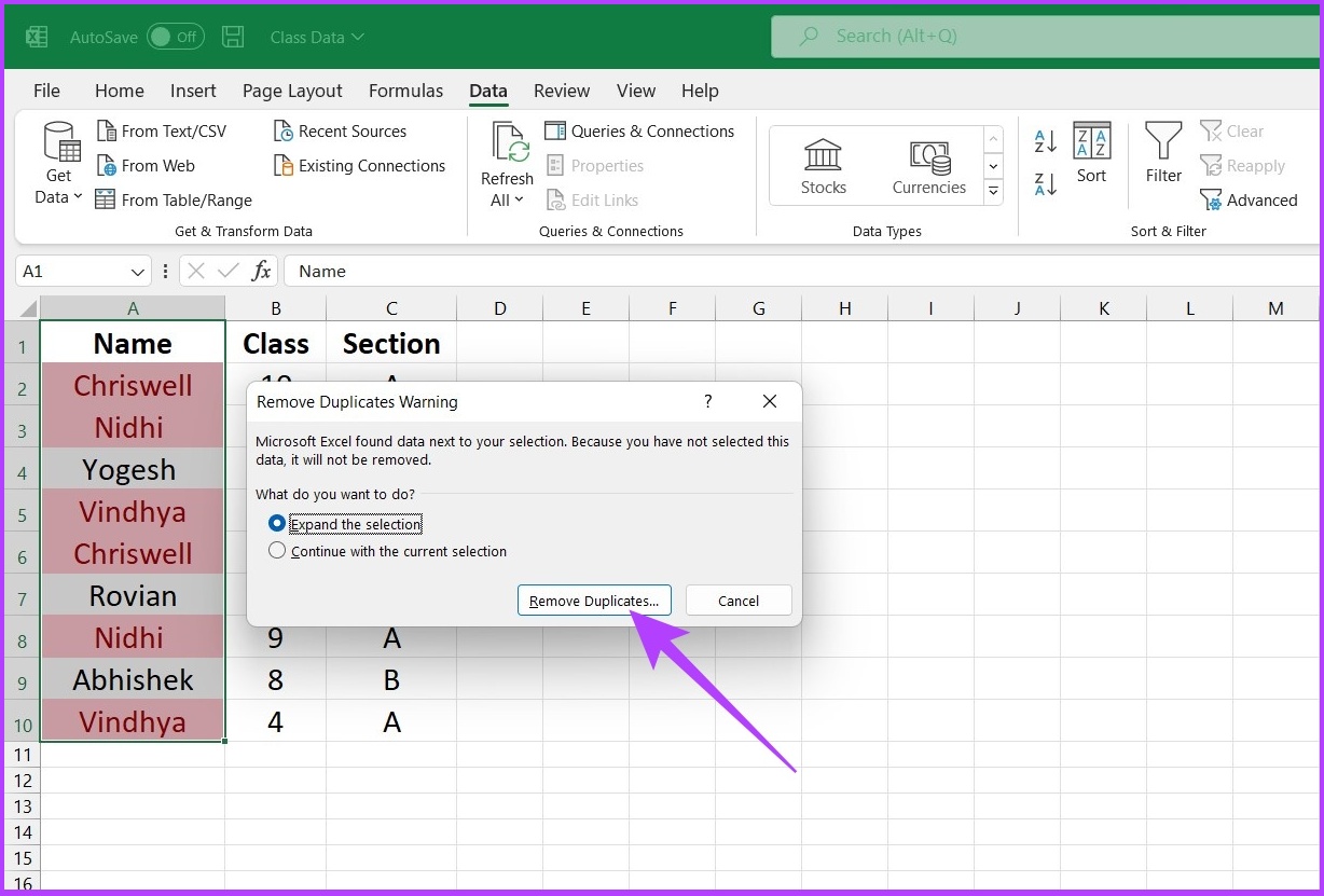
Step 4: In the Remove Duplicate Warning dialog box, select Expand the Selection and click on Remove Duplicates.
Step 5: Under Remove Duplicates, select duplicate columns you want to delete and click OK.
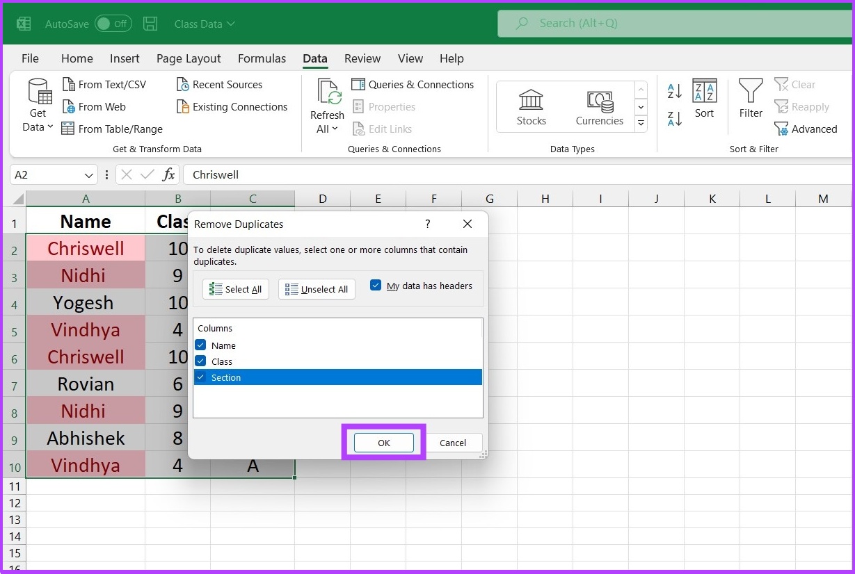
Excel will remove duplicate entries from the selected dataset and leave the unique data for your processing.

Duplicate-Free Unique Spreadsheet in Excel
Highlighting duplicate cell values will be a smart move if you’re dealing with a large dataset. The above-mentioned methods will help you for sure, irrespective of whether you use Excel regularly or occasionally. I hope this guide helped you in highlighting duplicates in Excel. Need more tricks to efficiently manage your work on Excel? Leave a thumbs up in the comment section below.
Was this helpful?
Last updated on 12 September, 2022
Read Next
 4 Fixes for Can’t Select or Highlight Text in Microsoft Word for Windows
Try Basic Fixes Rule out issues with your mouse or touchpad: A malfunctioning mouse or touchpad might fail to register clicks and drag motions.
4 Fixes for Can’t Select or Highlight Text in Microsoft Word for Windows
Try Basic Fixes Rule out issues with your mouse or touchpad: A malfunctioning mouse or touchpad might fail to register clicks and drag motions.
 Easy Ways To Fix Excel Not Responding or Slow
Why Does Excel Keep Freezing or Lags on Windows If the Excel app or file stops responding or lags, it can be attributed to various factors.
Easy Ways To Fix Excel Not Responding or Slow
Why Does Excel Keep Freezing or Lags on Windows If the Excel app or file stops responding or lags, it can be attributed to various factors.
 3 Ways to Insert an Excel Spreadsheet into a Word Document
Method 1: Using the Insert Table Option The Insert tab on the Word Ribbon has different options, including an Insert Table button, which can be used to insert an Excel
3 Ways to Insert an Excel Spreadsheet into a Word Document
Method 1: Using the Insert Table Option The Insert tab on the Word Ribbon has different options, including an Insert Table button, which can be used to insert an Excel
 3 Ways to Extract a URL From Hyperlinks in Microsoft Excel
Method 1: From the Edit Hyperlink Dialog The context menu has a series of shortcuts for performing actions.
3 Ways to Extract a URL From Hyperlinks in Microsoft Excel
Method 1: From the Edit Hyperlink Dialog The context menu has a series of shortcuts for performing actions.
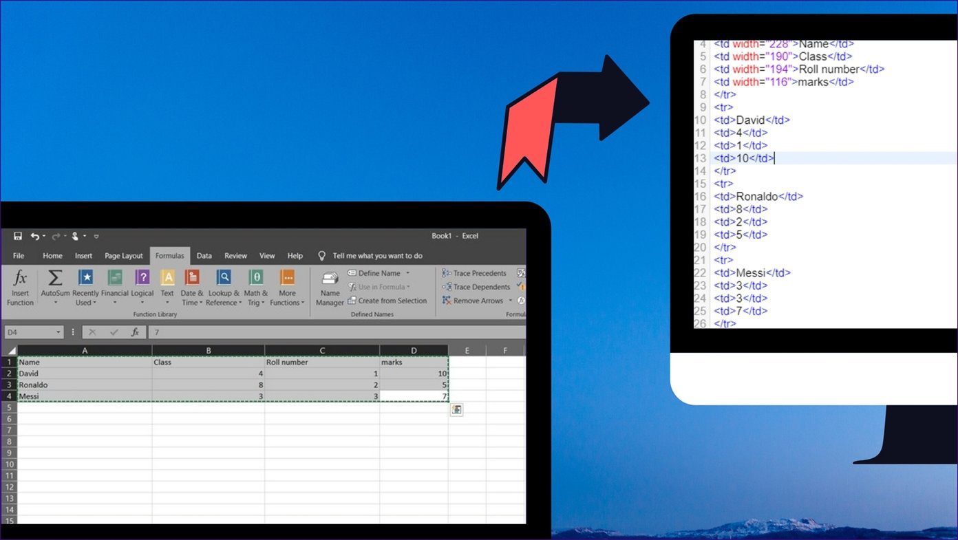 How to Convert an Excel Sheet to an HTML Table
Method 1: Save as Webpage Excel lets you save your documents in different formats.
How to Convert an Excel Sheet to an HTML Table
Method 1: Save as Webpage Excel lets you save your documents in different formats.
 How to Use Version History in Microsoft Excel
How to View Version History in Microsoft Excel for PC or Mac Accessing an older version of an Excel workbook on your PC or Mac only takes a few steps.
How to Use Version History in Microsoft Excel
How to View Version History in Microsoft Excel for PC or Mac Accessing an older version of an Excel workbook on your PC or Mac only takes a few steps.
 4 Fixes When Excel Worksheet Tabs Are Not Showing
Basic Fix: Resize Excel window: When you notice that the tabs of your Excel workbook are not visible, first confirm that other opened programs do not block the tabs.
4 Fixes When Excel Worksheet Tabs Are Not Showing
Basic Fix: Resize Excel window: When you notice that the tabs of your Excel workbook are not visible, first confirm that other opened programs do not block the tabs.
 How to Remove Table Formatting in Excel
Method 1: Clear Table Style When working with data tables, Excel often applies predefined styles that include various formatting elements such as colors, borders, and fonts.
How to Remove Table Formatting in Excel
Method 1: Clear Table Style When working with data tables, Excel often applies predefined styles that include various formatting elements such as colors, borders, and fonts.
The article above may contain affiliate links which help support Guiding Tech. The content remains unbiased and authentic and will never affect our editorial integrity.