Excel How to Format a Whole Row Based on One Cell

Quick Tips

• Conditional Formatting is generally one of the most versatile features of Excel, and it contains many features that we won’t cover due to brevity.
• Drop-down lists can also be used as Conditional Formatting criteria.
• Checkboxes are easy to format with, but Excel doesn’t have a way to enter and link them into multiple cells at a time.
• If your cells don’t format correctly, recheck to see if you’re using the correct reference types for rows and columns.

By default, conditional formatting in Excel allows you to format the cell’s look (such as font or background color) based on its own value. But by extending the range of the “check,” you can learn how to format a whole row based on one cell in it.

Part 1: Excel Format a Whole Row Based on One Cell Value

To make things a bit simpler to explain, we’ll have a sample table from B2 that displays employee information including when their contract ends. We’ll check if that date has past and format their entire row red.

For reference, here’s what an employee table might look like.

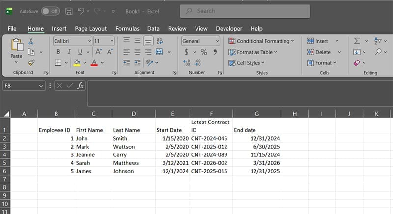
Step 1. Select the entire range where your data is (excluding the headers). In this case, we’re using B2:G6.

Step 2. Click on “Conditional Formatting” then select “New Rule.”

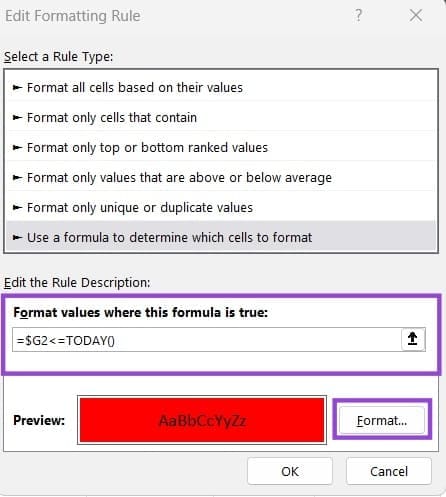
Step 3. Choose the option “Use a formula to determine which cells to format.”

Step 4. In the formula, we’ll use the function: =$G2<TODAY()

This formula will go through the entire table. Since the “G” column has a “$” before it, it will be locked to check the end date of the contract. The “row” indicator will move as the formula goes down the table, and needs to start with the first row where the data is (in this case 2).

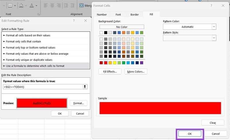
Step 5. Click on the “Format” button, then go to the “Fill” tab and choose the color to fill the cell with. You can also choose additional formatting if you want. When you’re happy with the choice, select “OK.”

Step 6. Click on “OK” in the Conditional Formatting menu to save the changes.

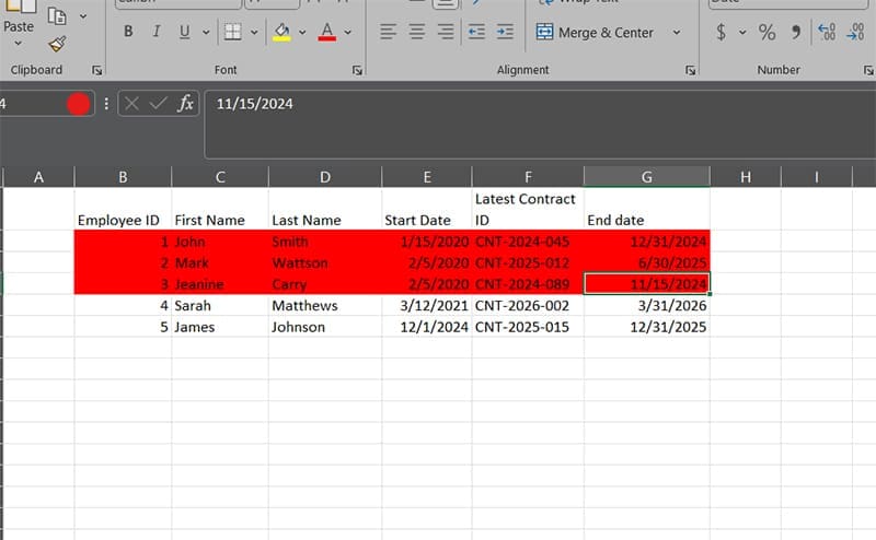
As a result, dates that have already passed (as of time of writing) as well as the entire row they’re in are highlighted.

If you want to combine multiple criteria, you can use the OR or AND functions, which have specific formatting requirements (such as OR(logical_test1,logical_test2…)). To search for a specific substring inside a cell, use the function =SEARCH(”string”,$ColumnRow)>0.

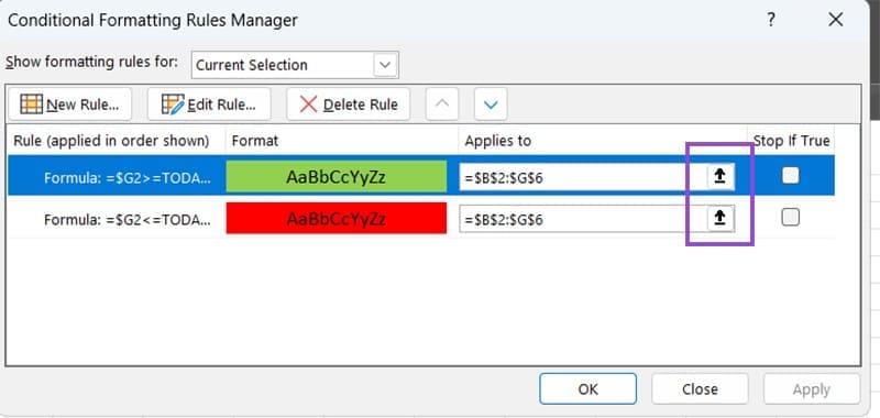
You can create multiple rules for the same table. In the above case, we created a rule to highlight all current contracts in green. Then, you can go to “Conditional Formatting” and “Manage Rules” to see all rules that apply to the table. Use the up and down arrows to change rule priorities (the last rule that is true will apply).

Part 2: How to Format a Row if a Checkbox Is Checked in Excel

Alternatively, for simple yes or no checks, you can implement checkboxes in cells that will act as logical “true” or “false” based on which to format the row.

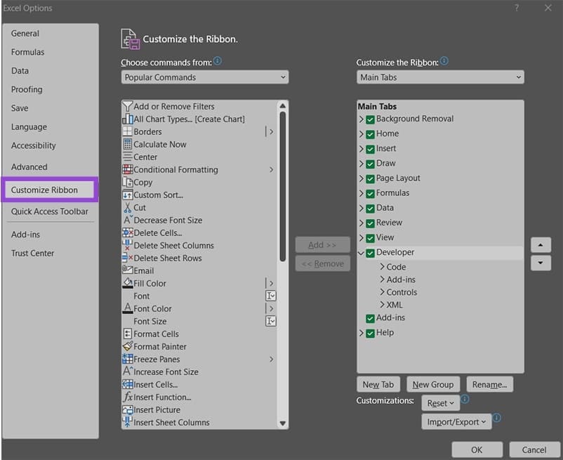
Notably, you’ll need to enable the Developer tab in Excel for versions that are not Excel 365 (which can be done via Options > Customize Ribbon > Enable the Developer box on the right panel).

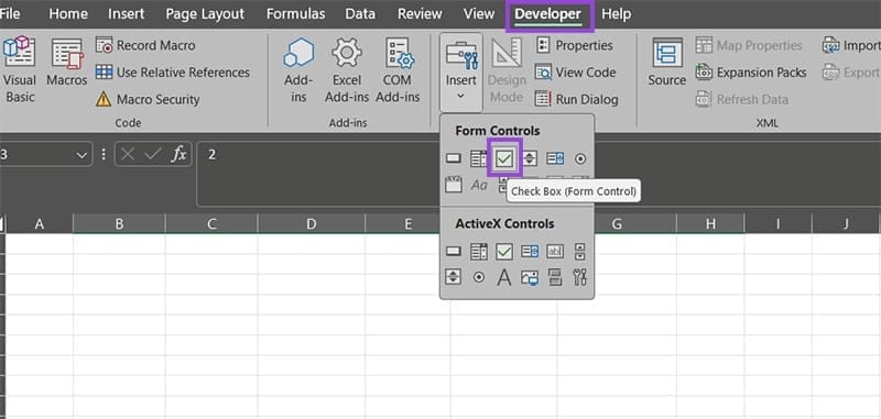
After that, you can add a checkbox to the table from the Developer tab from “Controls” then “Checkbox.” This places a checkbox on the table, which needs to be moved into place.

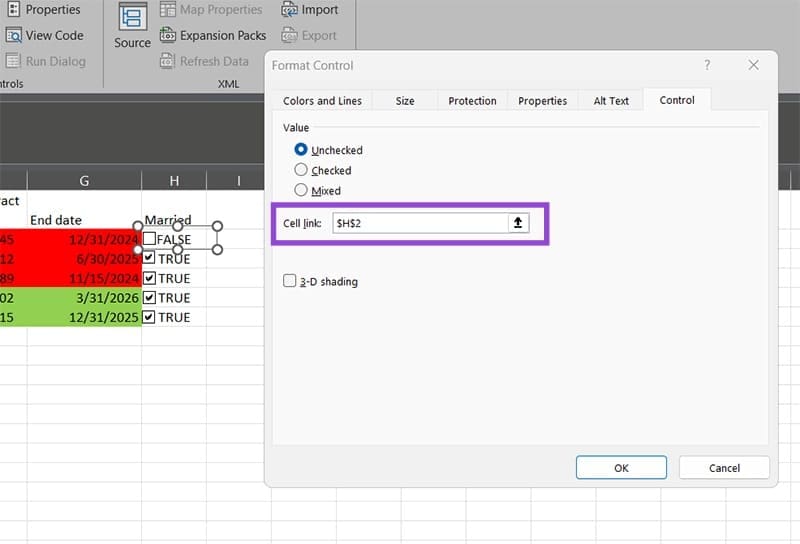
For this, we’ve added a column H to display an employee’s marital status.

Step 1. Add five checkboxes to the table. For each, remove the text, then right-click on it and select “Format Control.”

Step 2. In the “Control” tab, enter the absolute reference to the cell the checkbox is in (for example, the first box will be “$H$2”).

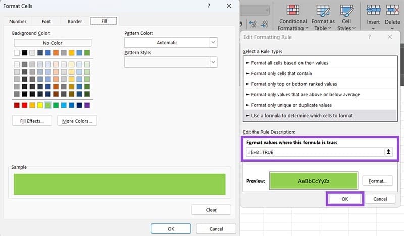
Step 3. Select the new table range and create Conditional Formatting. This time, the formula will be “=$H2=TRUE” since we’re using the H column.

Step 4. Select your formatting and click “OK” on both boxes.

We’ve removed the previous rules to make things easier to see.