10 Essential Microsoft Excel Functions for Data Analysis

Microsoft Excel offers users hundreds of different functions and formulas for a variety of purposes. Whether you have to analyze your personal finance or any large data set, it’s the functions that make the job easy. Also, it saves a lot of time and efforts. However, finding the right function for your data set can be very tricky.

So if you’ve been struggling to find the appropriate Excel function for data analysis, then you’ve come to the right place. Here’s a list of some essential Microsoft Excel functions that you can use for data analysis and you can boost your productivity in the process.

1. CONCATENATE

=CONCATENATE is one of the most crucial functions for data analysis as it allows you to combine text, numbers, dates, etc. from multiple cells into one. The function is particularly useful for combining data from different cells into a single cell. For instance, it comes handy for creating the tracking parameters for marketing campaigns, build API queries, add text to a number format, and several other things.

In the example above, I wanted the month and sales together in a single column. For that, I have used the formula =CONCATENATE(A2, B2) in the cell C2 to get Jan$700 as the result.

Formula: =CONCATENATE(cells you want to combine)

2. LEN

=LEN is another handy function for data analysis that essentially outputs the number of characters in any given cell. The function is predominantly usable while creating title tags or descriptions that have a character limit. It can also be useful when you’re trying to find out the differences between different unique identifiers which are often quite lengthy and not in the correct order.

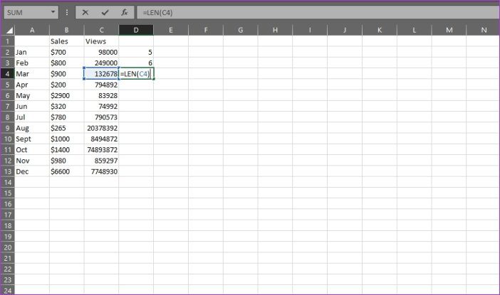
In the example above, I wanted to count the figures for the number of views I was getting each month. For this, I made use of the formula =LEN(C2) in the cell D2 to get 5 as the result.

Formula: =LEN(cell)

3. VLOOKUP

=VLOOKUP is probably one of the most recognizable functions for anyone familiar with data analysis. You can use it to match data from a table with an input value. The function offers two modes of matching — exact and approximate, which is controlled by the range of the lookup. If you set the range to FALSE, it’ll look for an exact match, but if you set it to TRUE, it’ll look for an approximate match.

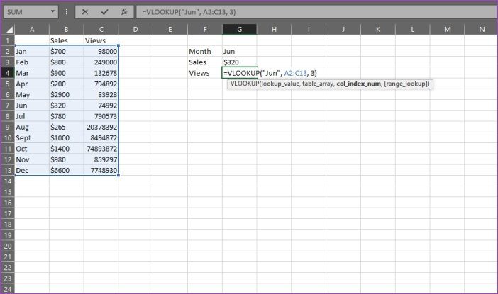
In the example above, I wanted to look up the number of views in a particular month. For that, I used the formula =VLOOKUP(“Jun”, A2:C13, 3) in the cell G4 and I got 74992 as the result. Here, “Jun” is the lookup value, A2:C13 is the table array in which I’m looking for “Jun” and 3 is the number of the column in which the formula will find the corresponding views for June.

The only downside of using this function is that it only works with data that has been arranged into columns, hence the name — vertical lookup. So if you’ve got your data arranged in rows, you’ll first need to transpose the rows into columns.

Formula: =VLOOKUP(lookup_value, table_array, col_index_num, [range_lookup])

4. INDEX/MATCH

Much like the VLOOKUP function, the INDEX and MATCH function come in handy for searching specific data based on an input value. The INDEX and MATCH, when used together, can overcome the VLOOKUP’s limitations of delivering the wrong results (if you are not careful). So when you combine these two functions, they can pinpoint the data reference and search for a value in a single dimension array. That returns the coordinates of the data as a number.

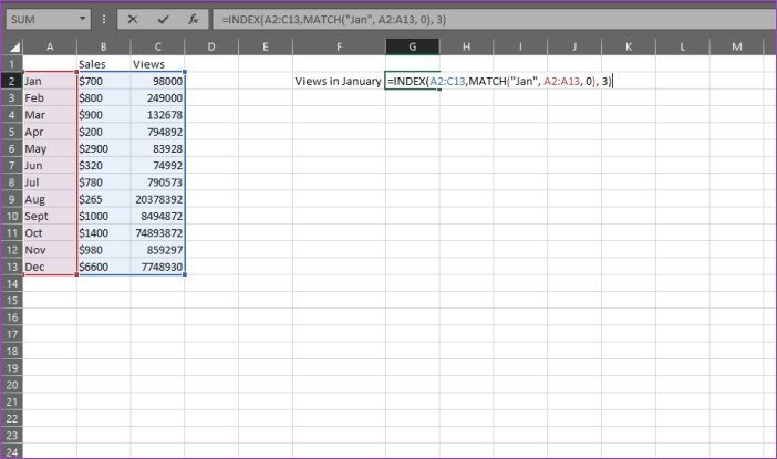
In the example above, I wanted to look up the number of views in January. For that, I used the formula =INDEX (A2:C13, MATCH(“Jan”, A2:A13,0), 3). Here, A2:C13 is the column of data I want the formula to return, “Jan” is the value I want to match, A2:A13 is the column in which the formula will find “Jan” and the 0 signifies that I want the formula to find an exact match for the value.

If you want to find an approximate match you will have to substitute the 0 with 1 or -1. So that the 1 will find the largest value less than or equal to the lookup value and -1 will find the smallest value less than or equal to the lookup value. Do note that if you don’t use 0, 1, or -1, the formula will use 1, by.

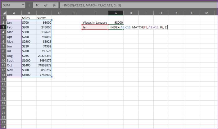
Now if you don’t want to hardcode the name of the month, you can replace it with the cell number. So we can replace “Jan” in the formula mentioned above with F3 or A2 to get the same result.

Formula: =INDEX(column of the data you want to return, MATCH(common data point you’re trying to match, column of the other data source that has the common data point, 0))

5. MINIFS/MAXIFS

=MINIFS and =MAXIFS are very similar to the =MIN and =MAX functions, except for the fact that they allow you to take the minimum/maximum set of values and match them on particular criteria as well. So essentially, the function looks for the minimum/maximum values and matches it with input criteria.

In the example above, I wanted to find the minimum scores based on the student’s gender. For that, I used the formula =MINIFS (C2:C10, B2:B10, “M”) and I got the result 27. Here C2:C10 is the column in which the formula will look for the scores, B2:B10 is a column in which the formula will look for the criteria (the gender), and “M” is the criteria.

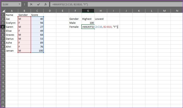
Similarly, for maximum scores, I used the formula =MAXIFS(C2:C10, B2:B10, “M”) and got the result 100.

Formula for MINIFS: =MINIFS(min_range, criteria_range1, criteria1,…)

Formula for MAXIFS: =MAXIFS(max_range, criteria_range1, criteria1,…)

6. AVERAGEIFS

The =AVERAGEIFS function allows you to find an average for a particular data set based on one or more criteria. While using this function, you should keep in mind that each criteria and average range can be different. However, in the =AVERAGEIF function, both the criteria range and sum range need to have the same size range. Notice the difference of singular and plural between these functions? Well, that’s where you need to be careful.

In this example, I wanted to find the average score based on the gender of the students. For that I used the formula, =AVERAGEIFS(C2:C10, B2:B10, “M”) and got 56.8 as the result. Here, C2:C10 is the range in which the formula will look for the average, B2:B10 is the criteria range, and “M” is the criteria.

Formula: =AVERAGEIFS(average_range, criteria_range1, criteria1,…)

7. COUNTIFS

Now if you want to count the number of instances a data set meets specific criteria, you’ll need to use the =COUNTIFS function. This function allows you to add limitless criteria to your query, and thereby makes it the easiest way to find the count based on the input criteria.

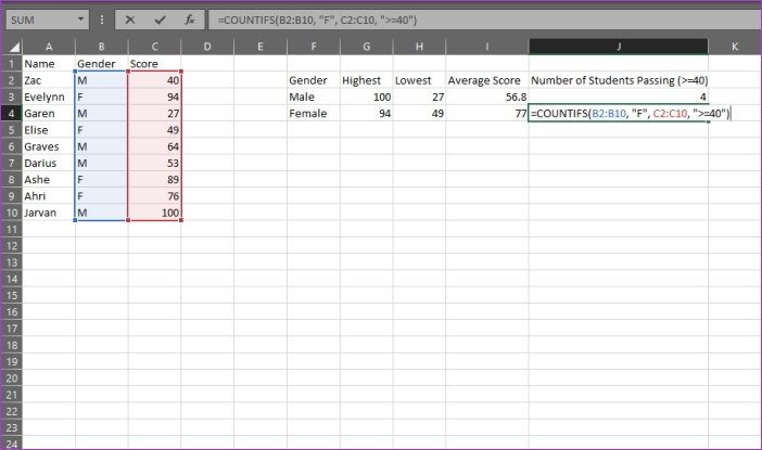
In this example, I wanted to find the number of male or female students who got passing marks (i.e. >=40). For that I used the formula =COUNTIFS(B2:B10, “M”, C2:C10, “>=40”). Here, B2:B10 is the range in which the formula will look for the first criteria (gender), “M” is the first criteria, C2:C10 is the range in which the formula will look for the second criteria (marks), and “>=40” is the second criteria.

Formula: =COUNTIFS(criteria_range1, criteria1,…)

8. SUMPRODUCT

The =SUMPRODUCT function helps you multiply ranges or arrays together and then returns the sum of the products. It’s quite a versatile function and can be used to count and sum arrays like COUNTIFS or SUMIFS, but with added flexibility. You can also use other functions within SUMPRODUCT to extend its functionality even further.

In this example, I wanted to find the sum total of all the products sold. For that, I used the formula =SUMPRODUCT(B2:B8, C2:C8). Here, B2:B8 is the first array (the quantity of products sold) and C2:C8 is the second array (the price of each product). The formula then multiples the quantity of each product sold with its price and then adds all of it up to deliver the total sales.

Formula: =SUMPRODUCT(array1, [array2], [array3],…)

9. TRIM

The =TRIM function is particularly useful when you’re working with a data set that has several spaces or unwanted characters. The function allows you to remove these spaces or characters from your data with ease, allowing you to get accurate results while using other functions.

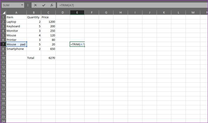
In this example, I wanted to remove all the extra spaces between the words Mouse and pad in A7. For that I used the formula =TRIM(A7).

The formula simply removed the extra spaces and delivered the result Mouse pad with a single space.

Formula: =TRIM(text)

10. FIND/SEARCH

Rounding things off are the FIND/SEARCH functions which will help you isolate specific text within a data set. Both the functions are quite similar in what they do, except for one major difference — the =FIND function only returns case-sensitive matches. Meanwhile, the =SEARCH function has no such limitations. These functions are particularly useful when looking for anomalies or unique identifiers.

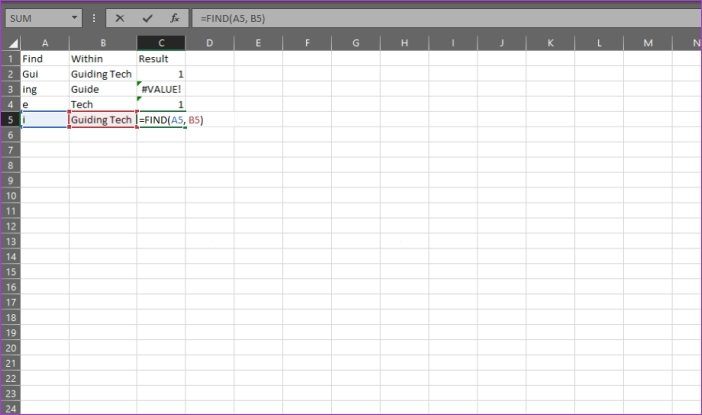
In this example, I wanted to find the number of times ‘Gui’ appeared within Guiding Tech for which I used the formula =FIND(A2, B2), which delivered the result 1. Now if I wanted to find the number of times ‘gui’ appeared within Guiding Tech instead, I’d have to use the =SEARCH formula because it isn’t case sensitive.

Formula for Find: =FIND(find_text, within_text, [start_num])

Formula for Search: =SEARCH(find_text, within_text, [start_num])

Master the Data Analysis

These essential Microsoft Excel functions will definitely help you with data analysis, but this list only scratches the tip of the iceberg. Excel also includes several other advanced functions to achieve specific results. If you’re interested in learning more about those functions, let us know in the comments section below.

Next up: If you wish to use Excel more efficiently, then you should check out the next article for some handy Excel navigation shortcuts that you must know.